Computer architecture can be considered a boring topic, one that is studied during CS education, then put aside, and leaves place to the shiny new toys that capture the attention.
I’ve recently revisited it, and I’d like to summarize some takeaways.

What is It

Computer architecture, like everything in the architecture and design domain, is concerned with building a thing, which here is a computer and all its components, according to requirements often called “-ilities”, such as cost, reliability, efficiency, speed, ease of use, and more.
Thus, it is inherently not limited to hardware, weight, power consumptions, and size constraints, but also includes taking into account decisions about design that fit a use-case within constraints.

Energy and Cost

Long gone are the days when we only cared about cramming more power in a single machine. We’ve moved to a world of battery-powered portable devices such as laptops and mobile phones. On such devices, we care about energy consumption as it directly affects battery life.

So what are some tips to avoid wasting energy.

• Do nothing well: As simple as it sounds it isn’t straight forward. We need to know when is the right time to deactivate a processor completely, otherwise we’ll pay a high penalty when putting it back online.
• Dynamic voltage-frequency scaling (DVFS): This is about changing the frequency of the processor’s clock, letting it consume instructions slower or faster. However, the same energy will be used for the same tasks, it’s just that the tasks will take longer to execute if the clock is slowed.
• Overclocking (Turbo mode): This is about boosting the power of a processor so that it executes more instructions, and so would finish tasks faster. You can notice the trade-off between either finishing tasks early and consuming more power, or taking time but finishing them later.
• Design for the typical case: Make the processor more efficient for the case that is the most frequent. Quite intuitive!

Keep in mind that these are all about dynamic power consumption, that is power consumption used by performing some actions, while in the background, there is always a static power consumption to keep the current system alive. Reducing static power consumption has an effect on the whole system.

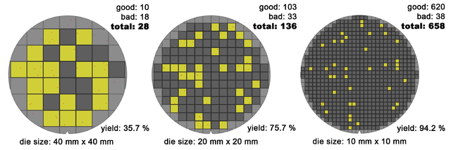
Similar to energy, cost is also important, because computers are now an everyday item. The cost of a microprocessor is in direct relation to the learning curve that companies have to take to build them, while on the other hand the price of DRAM actually tracks the cost of manufacturing. When we talk of microprocessors, we are talking about a composition of one or multiple die, which have their circuit printed by UV lithography on a wafer (photolithography). And so, the price is in relation to how many dies (square shaped) can fit on a wafer (circle shaped), along with the yield, which is the number of non-defective dies, plus the cost of testing them and packaging them.
This is one of the reason big companies focus on commodity hardware — hardware that’s relatively cheap and replaceable. Only in the case of specialized or scientific computing will we ever see costly, hard-to-replace, and custom pieces of hardware.

Dependability is also a big factor that comes into play: how long will the piece of hardware last. This is especially important in big warehouse. If we’re going to replace a cheap piece way more frequently than another one that is just a little bit more expensive, we may be better off choosing the second one. Technically, we talk of Mean Time To Failure (MTTF) and Mean Time To Repair (MTTR).

Measurements and Bottlenecks

You can’t talk without the numbers to prove it, that’s why measurement is everything. We’re talking about benchmarks for computer architecture, similar to Phoronix-style benchmarks.
There are many ways to measure, report, and summarize performance, and different scenarios in which they apply. These aren’t limited to pure crunching of numbers, but benchmarks can go as far as to simulate kernels, desktop behaviors, and web-servers. Three of the most important ones are the EEMBC, which is a set of kernels used to predict hardware performance, the TPC benchmarks which are directed towards cloud infrastructures, and the SPEC family of benchmarks which touch a bit of everything.
Many of the results of these benchmarks are proprietary and/or costly.

Measuring is important because we want to make sure our most common case is fast. That’s a fact that comes out of something called Amdahl’s Law. Simply said, if you optimize a portion of code that is only used 1% of the time you’ll only be able to have a maximum speedup of 1%.
Additionally, we should also check if we can parallelize computation in the common case, and if we can apply the principle of locality to it, that is reuse data and instructions so that they stay close temporally and physically.

ISA — Instruction Set Architecture

As much as people freak out about assembly being low-level, it is still a language for humans (not machines) that requires another software, called an assembler, to be converted to actual machine code instructions. However, it is most often tied to the type of instructions a machine can process — what we call the instruction set architecture, or ISA for short. That is one reason why we have many assembly flavors: because we have many ISAs.

To understand the assembly flavor you are writing in, it’s important to know the differences and features of the ISA, and if additional proprietary options are provided by the manufacturer. These can include some of the following.

• The classification of ISA: Today, most ISAs are general-purpose register architectures, that means operands can either be register or memory location. There are two sub-classes of this: the register-memory ISAs, where memory can directly be accessed as part of instructions, like 80×86, and load-store ISAs, where memory can only be accessed through load and store operations, like ARMv8 and RISC-V. Let’s note that all new ISAs after 1985 are load-store.

• The way the memory is addressed: Today, all ISAs point at memory operands using byte addressing, that means we can access values in memory by byte, in contrast with some previous ISAs where we had to fetch them by word (word-addressable). Additionally, some architectures require that objects be aligned in memory, or encourage users to align them for efficiency reasons. In ARMv8 they must be aligned, and in 80×86 and RISC-V it isn’t required but encouraged.

• The modes in which memory can be addressed: We know that the operand to address memory has to be bytes but there are many ways to precise how to get them. We could get a value by pointing to the address stored in a register, or by pointing to the value stored at the immediate address of a constant, or to the value stored at the address formed by the sum of the value of a register plus a constant (displacement). These 3 modes are available in RISC-V. 80×86 adds other modes such as: no register (absolute), getting the address from one register as an index and another register the displacement, and from two registers where one register is multiplied by the size of the operand in bytes, and more. ARMv8 has the 3 RISC-V modes plus PC-relative addressing, the sum of two registers, and the sum of two registers where one registers is multiplied by the size of the operands in byte. Yes, there are so many ways to give an address in memory!

• Types and size of operands/data/registers: An ISA can support one or multiple types of operands ranging from: 4-bit (nibble), 8-bit, 16-bit (half word), 32-bit (integer or word), 64-bit (double word or long integer), and in the IEEE-754 floating-point we can have 32-bit (single precision), 64-bit (double precision), etc. 80×86 even supports 80-bit floating-point (extended double precision).

• The type of operations available: What can we do on the data, can we do data transfer, arithmetic and logical operations, control flow, floating-point operations, vector operations, etc. 80×86 has a very large set of operations that can be done. Let’s also note that some assembly flavors include the type of operands within the operations and thus new instructions need to be added for new types (see under CISC).

• The way control flow instructions work: All ISAs today include at least the following: conditional branches, unconditional jumps, and procedure calls and returns. Normally, the addresses used with those are PC-related. On RISC-V, the condition for the branch is checked based on the value content of registers, while on 80×86, the test condition code bits are set as side effects of previous arithmetic/logic operations. As for the return address, on ARM-v8 and RISC-V, it is placed in a register, while on 80×86, it is placed on the stack in memory. This is one of the reason stack overflows on 80×86 are so dangerous.

• Encoding the ISA instructions: Finally, we have to convert things to machine code. There are two choices in encoding: with fixed length or with variable length. ARM-v8 and RISC-V instructions are fixed at 32-bit long, which simplifies instruction decoding. 80×86, on the other hand, has variable length instructions ranging from 1 to 18 bytes. The advantage is that the machine code takes less space, and so the program is usually smaller. Keep in mind that all the previous choices affect how the instructions are encoded into a binary representation. For example, the number of registers and the number of addressing modes need to be represented somehow.

Moreover, ISAs are grossly put into two categories, CISC and RISC, the Complex Instruction Set Computer and Reduced Instruction Set Computer.
RISC, are computers with a small, highly optimized set of instructions, with numerous registers, and highly regular instruction pipeline. Usually, RISCs are load-store architectures with fixed size instruction encoding to keep the clock cycle per instruction (CPI) constant.
CISC, are computers with a very large set of instructions, instructions which can execute several lower-level operations, can have side effects, can access memory through a single instruction that encompasses multiple ones, etc. It englobes anything that isn’t RISC or that isn’t a load-store architecture.

It has to be said, that different manufacturers can implement one ISA differently than others. Which means, that their implementation can consume the same instruction encoding but that the actual hardware is different. ISAs are like the concept of interfaces in OOP.

Memory Hierarchy and Tech

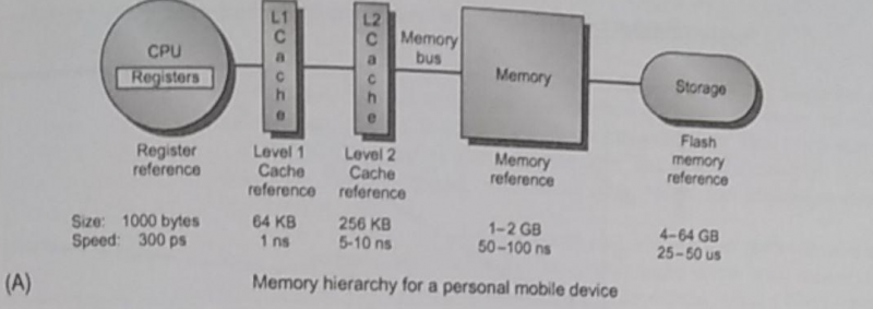
Many authors have written a great deal about memory hierarchy, basically it’s all about creating layers of indirection, adding caches to speed things up at each layer, wanting to keep what we’re going to use close temporally and physically, while having in consideration how the layers are going to be used.
For example, the associativity of an L2 instruction cache might not be as effective when applied to an L2 data cache. When in doubt, refer to the benchmark measurements.

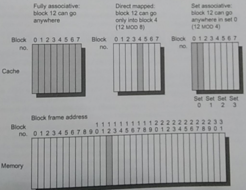
There are four big questions that we should ask at each layer:

• Where can a block be placed
• How is a block found if it is there
• Which block should be replaced on a miss
• What happens on a write

With these, there’s also an interplay with both the lower and upper layers. For instance, issues like the size and format of cached lines when they have to be moved up or down between the caching layers.
Additionally, synchronization and coherence mechanisms between multiple caches might be important.

When it comes to data storage, the hardware speed, its ability to retain information, its power consumption, its size, and other criteria, are what matters. Let’s review some common technologies in use today.

Static RAM, or SRAM, has low latency and requires low power to retain bits, however for every bit at least 6 transistors are required. It’s normally used in processor cache and has a small storage capacity.
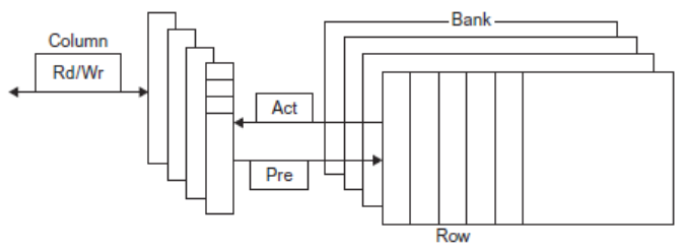
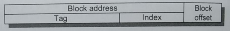
Dynamic RAM, or DRAM, is slower but requires only one transistor per bit. However, it has to both be periodically refreshed (every ~8ms) and must be re-written after being read. DRAM is usually split into rows and columns, where the upper half of the address is found in the row and the lower in the column, we talk of row access strobe (RAS) and column access strobe (CAS). It is normally used as the main memory.
Because DRAM is cheaper to manufacture, to make it more profitable, it has received a lot of improvements to face its limitations. For example, some of the optimization are related to bandwidth. Namely, double data rate allows transferring twice per clock signal, and multiple banks allow accessing data in different places at the same time. Multiple banks are key to SIMD (see under Single Instruction Multiple Data Stream).

Flash memory technology, aka EEPROM, be it NAND or NOR gated, is becoming popular as a replacement for hard disk drives because of its non-volatility and low power. It can act as a cache in between the disk and the main memory. It has its own limitation in the way it updates by blocks.
Some of the latest hype is about Phase Change Memory (PCM or PRAM), which is a type of nonvolatile memory that is meant as a replacement for flash memory but that is more energy efficient.

However, we can’t rely on the physical medium alone to bring all the improvements. Some techniques have to be put in place to make the most out of what we got.

Efficiency doesn’t matter if the medium fails. All these beautiful hardware can fall victim to two types of errors: soft errors, which can be fixed by error correcting codes (ECC), and hard errors, which make the section of data defective, requiring either redundancy or replacement to avoid data loss. Beware of cosmic rays!

Effectiveness can also be found in the layout and architecture used for caching. Here are some interesting questions that can be answered by performing benchmarks for the use-case. Remember, that everything is about trade-offs.

• Should we use large block size to reduce misses that are caused by the block not being already there. However, that would also increase conflict miss (two blocks that collide because of their addresses in the cache) and miss penalty time (the time spent to fetch a block when it isn’t already there).
• Should we enlarge the whole cache to reduce miss rate. However, it would increase the hit time (time to find the cache line) and power consumption.
• Should we add more cache levels, which would reduce the overall memory access time but increase power consumption and complexity, especially between caches.
• Should we prioritize read misses over write misses to reduce miss penalty, does it fit our case.
• Should we use multiple independent cache banks to support simultaneous access, or does it add complexity.
• Should we make the cache non-blocking, allowing hits before previous misses complete (hit under miss).
• Should we merge the write buffers that has writes to the same block to avoid unnecessary travel or would that slow writes.
• Should we rely on compiler optimizations that take in consideration the locality of the cache such as loop interchange (change the loop so that memory is accessed in sequential order), and subdividing the loops into small matrices that fit into the cache. Or would that behavior confuse the cache and actually have an opposite effect.
• Should we use/have prefetching instructions if the ISA allows it to fill the cache manually or would that let the compiler mishandle the cache and fill it with unnecessary garbage, throwing away the locality of other programs.

These are all questions that can’t be answered without actual benchmarks.

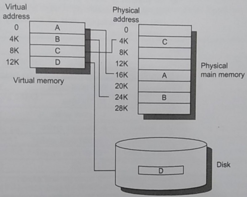
For processes, there’s never enough space in the main memory. In multi-programming systems, the OS virtualizes access to memory, for both simplicity, space restriction, and security reasons. Each process thinks it’s running alone on the system.
The same four questions about memory placement applies. Particularly, the OS is the one who decides what to do with each piece, or page, of virtual memory. A page being the unit of manipulation, and often being the same size as a disk sector.
This means that there’s another layer of addresses, virtual ones, that need to be translated to physical ones, and that the OS needs to know where that pages currently are: either on the disk or in main memory.
For a faster translation, we could use a cache sitting near the core that would contain the recent translated addresses, a so-called translation buffer or translation look aside buffer (TLB).

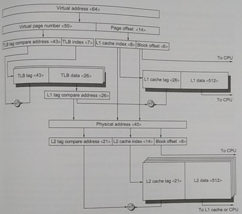
Additionally, if the virtual address can be composed in a way that doesn’t require going back to memory to fetch the data, but can be used to point to the data directly, in another cache for example, then the translation can be less burdensome.

Virtual memory can also be extended with protection, Each translation entry we can have extra bits representing permission or access rights attributes. In practice, there are at least two modes: user mode and supervisor mode. The operating system can rely on them to switch between kernel mode and user mode, limiting access to certain memory addresses and other sensitive features, a dance between hardware and software.

Virtual memory is the technology that makes virtual machines a reality. A program called a hypervisor, or virtual machine monitor, is responsible to manage virtual memory in such a way that different ISAs and operating systems can run simultaneously on the same machine without polluting one another. It does it by adding a layer of memory called “real memory” in between physical and virtual memory. Optimizations such as having the TLB entries not constantly flush when switching between modes, having virtual machine guests OS be allowed to handle device interrupts, and more are needed to make this tolerable.

Parallelism

Parallelism allows things to happen at the same time, in parallel. There are two classes of parallelism: Data-Level Parallelism (DLP), and Task-Level Parallelism (TLP). Respectively, one gives the ability to execute a single operation on multiple pieces of data at the same time, and one to effectuate multiple different operations at the same time.
Concretely, according to Flynn’s taxonomy, we talk of Single-Instruction stream Single-Data stream (SISD), Single-Instruction stream Multiple-Data stream (SIMD), Multiple-Instruction stream Single-Data stream (MISD), and Multiple-Instruction stream Multiple-Data stream (MIMD).

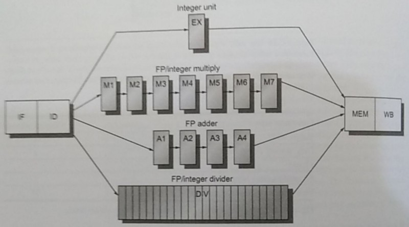
None of these would be possible without the help of something called pipelining. Pipelining allows instructions to be overlapped in execution by splitting them into smaller pieces that can be run independently, and that together form a full instruction. It is like a car assembly line for instructions, we keep fetching instruction on each lane and push them down at each step.
A typical breakdown of an instruction goes as follows:

• Instruction fetch
• Instruction decode and register fetch
• Execution or effective address cycle
• Memory access
• Write-back

That means with 5 lanes we should possibly be able to execute 5 instructions per clock cycle. However, the world isn’t perfect, and we face multiple major issues that don’t make this scenario possible: Hardware limitations, such as when we have a specific number of units that can perform the current step (structural hazards), when the data operands of instructions are dependent on one another (data hazards), when there are branches in the code, conditions that should be met for it to execute (control hazards). Another thing to keep in mind is that some instructions may take more than one cycle to finish executing and so may incur delay in the pipeline.

The data hazards category can be split into 3 sub-categories:

• Read after write (RAW): When data needs only to be read after it has been written by another instruction.
• Write after read (WAR): When data needs to be written only after another instruction has finished reading it.
• Write after write (WAW): When data needs to be written only after another has written to it.

Many ingenious techniques have been created to avoid these issues. From stalling, to data forwarding, finding if the data dependence is actually needed, renaming variables in registers to virtual registers, to loop unrolling, and more.

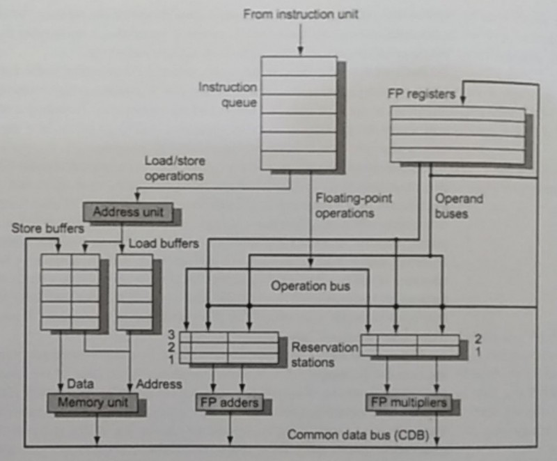
Virtual registers is a technique used in dynamic scheduled pipelines aka dynamic scheduling. Unlike in-order instructions where we have to wait for long-running instructions to finish for another one that may or may not depend on it to be processed, dynamic scheduling uses out-of-order instructions and solves the dependencies internally. Popular algorithms are scoreboard, Tomasulo’s, and the reorder buffer (ROB).
These algorithms achieve the out-of-order execution by relying on additional hardware structures to store values that could possibly, when certain of the output, write them back to memory.

The hazards that affect performance the most are control hazards. Because of their conditional aspect, whether a branch is taken or not, we either have to freeze the pipeline until we know if it’s taken, or we choose to continue loading instructions from one of the path and flush them if the branch wasn’t actually taken.
What we can do to reduce the cost of branches is to try to predict, to speculate, through hardware or software/compiler. The compiler can do a Profile-Guided Optimization (POG), running the software and gathering information about which branches are taken the most frequently, to then indicate it, one way or another, in the final binary. As far as hardware goes, past behavior is the best indicator of future one, and so instruction cache can have their own prediction mechanism based on previous values. Some well-known algorithms: 2-bit prediction, tournament predictor, tagged-hybrid predictor, etc.

In all these cases, we need to pay close attention to what is executed; we shouldn’t execute instructions from a branch that wasn’t supposed to be taken, notably in the case where it’ll affect how the program behaves. However, in speculative instructions and dynamic scheduling, we allow executing future instructions from any branch as long as the code doesn’t have an effect. We then face a problem when it comes to exceptions in instructions that weren’t supposed to be executed, how do we handle them. It depends on the types of exceptions if we terminate or resume execution. But handling exceptions can be slow, thus some architecture provide two modes, one with precise exception and one without for faster run.

Another way to speed instructions is to issue more of them at the same time. Some of the techniques in this category put more emphasis on hardware, like statically and dynamically scheduled superscalar processors or increasing the fetch bandwidth, while others rely on the software/compiler: such as very long instruction word (VLIW) processors, which packages multiple instructions into one big chunk that is fetched at the same time.

Sometimes, whole chunks of code are independent, and so it would be advantageous to run them in parallel. We do that with multithreading, thread-level parallelism, a form of MIMD because we both execute different instructions on shared data between threads. In a multiprocessor environment, we can assign n threads to each processor.
There are 3 categories of multithreading scheduling:

• Fine grained multithreading: When we switch between threads at each clock cycle.
• Coarse grained multithreading: When we switch between threads only on costly stalls.
• Simultaneous multithreading (SMT): Fine grained multithreading but with the help of multiple issue (issuing multiple instructions at the same time).

There are two ways to lay the processors in an architecture, and it directly affects multithreading, specially when it comes to sharing data.

• Symmetric multiprocessors (SMP): In this case we have a single shared memory, the processors are equidistant, and so we have uniform memory latency.
• Distributed shared memory (DSM): In this case the processors are separated by other types of hardware, the memory distributed among processors, the processors may not be at the same distance from one another, and so we have a non-uniform memory access (NUMA).

In thread-level parallelism the bottleneck lies in how the data is synchronized between the different threads that may live in different processors — it is a problem of cache coherence and consistency.
The two main protocols to solve this are directory based, which consists of sharing the status of each block kept in one location, usually the location is the lowest level cache L3, or snooping, which consists of each core tracking the status of each block and notify others when it is changed.
Along with these, we need ways to handle conflicts between thread programmatically, and so processors offer lock mechanisms such as atomic exchange, test-and-set, and fetch-and-increment.

Let’s now move our attention to another type of parallelism: SIMD, data level parallelism.

SIMD adds a boost to any program that relies heavily on doing small similar operations on big matrices of data, such as in multimedia or scientific applications.
We note 3 implementations of SIMD:

• Vector architectures: They have generic vector registers, like arrays that can contain arbitrary data and where we can specify the size of operands in the vector before executing an instruction.
• SIMD extensions (Intel MMX, SSE, AVX): It is a bunch of additional instructions added as an afterthought to handle SIMD related data, they have fixed size for each operand, the number of data operands are encoded in op code, there are no sophisticated addressing modes such as strided or scatter-gather, and mask registers are not usually present.
• GPU: A specialized proprietary unit that can receive custom instructions from the CPU to perform the single operation on data heavy input.

All of these provide instructions to the compiler that more or less act like this: Load an array in a vector register only specifying the start address and size, operate on that special vector register, and finally push back the result into memory.
Some architectures provide ways to apply the instructions conditionally on the data in the vector register by specifying a bit mask. But beware of loading a whole dataset for a bit mask that only applies to a very small portion of the code. Vector instructions, like all instructions have a start up time, a latency that depends on the length of the operands, structural hazards, and data dependencies.
Another feature that some provide is the scatter-gather, for when array indices are represented by values present in another array.

Memory banks are a must for SIMD because we operate intensively on data that could be in multiple places. This is why we need support for high bandwidth for vector loads and stores, and to spread accesses across multiple banks.

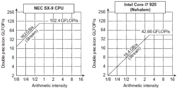
We measure performance in SIMD by using the concept of roofline, a performance model. It calculates graphically when we reach the peak performance of our hardware, the more left oriented the peak is, the more we’re using out of our hardware.

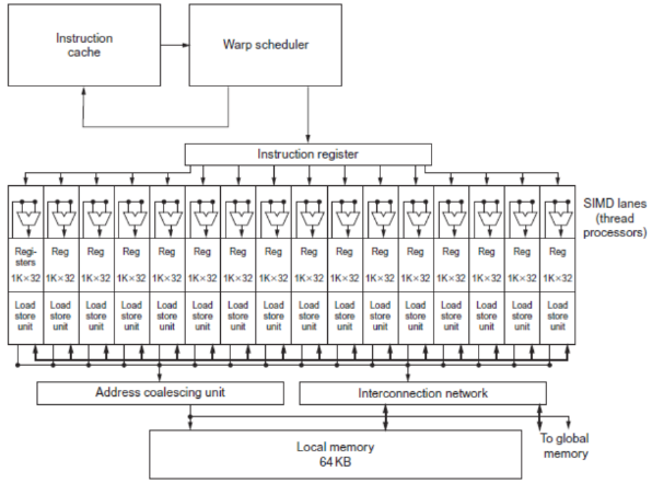
GPUs are beasts of their own, specialized in only SIMD instructions. They’re part of a heterogeneous execution model, because we have the CPU as host and the GPU as an external device that is requested to execute instructions.
Interacting with GPU differs between vendors, some standards exists such as OpenCL but are not widely used. Normally, it’s a C-like programming language that is made easy to represent SIMD. However, we sometimes call them Single-Instruction Multiple-Thread because GPUs are internally composed of hundreds, and sometimes thousands, of threads, often called lanes in GPU parlance.

GPUs are insanely fast because they have a simple architecture that doesn’t care about data dependence or other hassle that normal processors have to deal with.

To make SIMD productive we have to use it properly by finding portions of code that can be executed with these instructions. Compilers are still struggling to optimize for data-level parallelism, loop-level algorithms can be used to try to find if array indices can be represented by affine functions, and then deduce more information from this. This is why multimedia libraries rely on assembly written manually by developers.

Big Warehouses

When architecture is applied at big scales, at warehouse scale, we have to think a bit differently. Today, the world lives in the cloud, from internet providers, to data centers, and governments, all have big warehouses full of computers.
Let’s mention some things that could be surprising about warehouse scale computing.

• At this scale, the cost against performance matters a lot.
• At this scale energy efficiency is a must, as it translates into power-consumptions and monthly bills.
• At this scale dependability via redundancy is a must, we have so many machines that at least one component is bound to fail every day. The hardware should also be easily replaceable.
• At this scale high network I/O is a must. Gigantic amount of money is put on switches and load balancers.
• At this scale we have to think about the cost of investment, the CAPEX (capital expenditures) and OPEX (operational expenditures), the loan repayment for the construction of the datacenter, and the return on investment (ROI).
• At this scale, we have to think wisely about the location we choose for the data center, be it because of cooling issues, of distance to the power-grid, of the cost of acquiring the land, distance to internet lines, etc.

In warehouses, we apply request-level parallelism, the popular map/reduce model.

And this is it for this article, one thing I haven’t mentioned but that is getting more traction, are domain specific architectures — custom processors made for special cases such as neural network, encryption, cryptocurrency, and camera image processing.

Conclusion

This was a small recap of topics related to computer architecture. It was not meant as a deep dive into it but just a quick overview targeted at those who haven’t touched it in a long time or that are new to it.
I hope you’ve at least learned a thing or two.
Thank you for reading!

References:

• Computer Architecture: A Quantitative Approach (The Morgan Kaufmann Series in Computer Architecture and Design) 6th Edition

Attributions:

• Internet Archive Book Images / No restrictions
• Wafer_die's_yield_model_(10-20-40mm).PNG: Shigeru23derivative work: Cepheiden / CC BY-SA (https://creativecommons.org/licenses/by-sa/3.0)
• 2x910 / CC BY-SA (https://creativecommons.org/licenses/by-sa/4.0)

If you want to have a more in depth discussion I’m always available by email or irc. We can discuss and argue about what you like and dislike, about new ideas to consider, opinions, etc..
If you don’t feel like “having a discussion” or are intimidated by emails then you can simply say something small in the comment sections below and/or share it with your friends.